Responsible AI for Developers Blog: Open Buildings Dataset: Downloading the Data

Open Buildings Dataset: Downloading the Data

November 18, 2022

Posted by Oscar Wahltinez, Developer Programs Engineer

Earlier this year, we announced the release of the Open Buildings dataset: a dataset of building footprints to support social good applications. And just a few weeks ago, we announced an update increasing the dataset coverage. This blog post will cover how to access this dataset for your own use cases.

An interactive map is available in the open buildings dataset site.

What's in the dataset? The dataset contains 817M building polygons and associated metadata. You can refer to the data format section of the open buildings dataset site for the full details, but here are some of the interesting bits:

The confidence field can be used to filter out low-confidence detections, or to perform weighted sampling depending on your applications.

If you only care about the centroid, you can skip the polygon altogether and use the latitude and longitude fields.

The geometry field describes the building footprint using the WKT (well-known text) format.

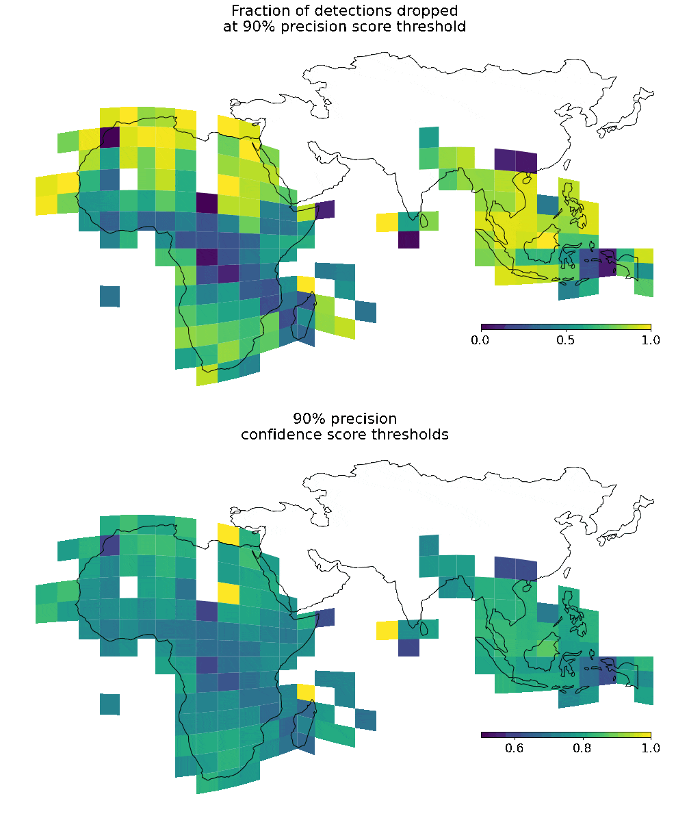
Geographical coverage As stated in the open buildings site, the dataset covers 64% of the African continent. Some areas have lower confidence detections than others, as illustrated in the FAQ section:

Moving image showing overall data coverage and 90% confidence building detection coverage

Visualization of overall data coverage and 90% confidence building detection coverage.

This means that, depending on the region of interest, you should use different thresholds to filter high-confidence detections.
Downloading compressed CSV files

As explained in the download data section of the open buildings dataset site, the data is available in a number of different files. Each individual file corresponds to an S2 cell at level 4. S2 cells are a fascinating concept, and we at Google use them quite a bit! If you want to read up more on it, check out the S2 geometry website for more information. In essence, S2 cells are a mathematical mechanism that helps computers translate Earth's spherical 3D shape into 2D geometry.

However, knowledge of S2 cells is not strictly required to use this dataset. This illustration tells you everything you need to know in order to download the data relevant to your region of interest:

Map of EMEA showing all areas covered by the dataset across Africa and South East Asia

Map with all areas covered by the dataset.

One small problem here is that most researchers are normally interested in specific administrative boundaries for data analysis. Fortunately, this Colab demonstrates how you can use the boundaries provided by Natural Earth (at low and high resolution) or World Bank. If you just want to download the data for an individual cell, it's quite simple! The library pandas natively supports reading compressed CSV files:

import pandas as pd

url_root = 'https://storage.googleapis.com/open-buildings-data/v1'

df = pd.read_csv(f'{url_root}/polygons_s2_level_4_gzip/1e9_buildings.csv.gz')

If you are only interested in the location of each building, rather than its footprint geometry, you can actually very efficiently load the entire open buildings dataset into memory. The following snippet takes about 10 minutes to run on a modest machine with 8 or more cores:

import concurrent.futures

import functools

import io

import pandas as pd

import tensorflow as tf

from tqdm.notebook import tqdm

def read_pandas_csv(url, **read_opts):

# This method is significantly faster for reading files stored in GCS.

with tf.io.gfile.GFile(url, mode='rb') as f:

return pd.read_csv(io.BytesIO(f.read()), **read_opts)

# Get all S2 cell tokens that contain buildings data.

# NOTE: Reading files directly from GCS is faster than the http REST endpoint.

url_root = "gs://open-buildings-data/v2"

# url_root = "https://storage.googleapis.com/open-buildings-data/v2"

tokens = read_pandas_csv(f"{url_root}/score_thresholds_s2_level_4.csv").s2_token

# The polygon type can be "points" (centroid) or "polygon" (footprint).

poly_type = "points" #@param ["points", "polygons"]

# Create a list with all URLs that we must download data from.

fnames = [f"{token}_buildings.csv.gz" for token in tokens]

poly_path = f"{url_root}/{poly_type}_s2_level_4_gzip"

urls = [f"{poly_path}/{fname}" for fname in fnames]

# Create a function that reads only a subset of fields given a URL.

columns = ["latitude", "longitude", "confidence"]

read_opts = dict(usecols=columns, compression='gzip')

map_func = functools.partial(read_pandas_csv, **read_opts)

with concurrent.futures.ThreadPoolExecutor(max_workers=8) as executor:

futures = [executor.submit(map_func, url) for url in urls]

completed = tqdm(concurrent.futures.as_completed(futures), total=len(futures))

table_iter = (future.result() for future in completed)

df = pd.concat(table_iter, copy=False, ignore_index=True)

The peak memory usage of that code is approximately 38GB (pro-tip: you can track that using the /usr/bin/time -v command), which sadly is larger than the maximum memory allocated to free Colab instances. While it's certainly possible to reduce the memory usage, it will likely come at the cost of speed.

Downloading Earth Engine FeatureCollection

Another way of accessing this dataset is by accessing the table available in the Earth Engine catalog in the form of a FeatureCollection. Generally speaking, you can access a feature collection trivially using the Earth Engine API:

import ee

# This only needs to be done once in your script.

ee.Authenticate()

ee.Initialize()

# Read the building polygons feature collection as-is.

buildings = ee.FeatureCollection('GOOGLE/Research/open-buildings/v2/polygons')

Although the above code finishes running almost immediately, the data has not been loaded into memory. To actually do something with this data, you have to either fetch it into the client or perform server-side operations. For more information, see the client vs server guide from Earth Engine.

You can take a peek at the first few by reading the feature collection client-side like this:

buildings.limit(10).getInfo()

Code and data availability

The code used in this blog post is available as part of the following Github repositories and gists:

https://gist.github.com/owahltinez/e1df3c41f0c90c54fe3546c5118ca019

Responsible AI for Developers Blog

Featured Post

Developer's Guide to Responsible AI

Open Buildings Dataset: Downloading the Data

More Information